A. geometric data
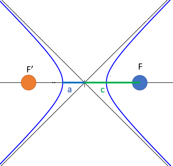
Hyperbole is an open conical plane. It is defined by the same geometric parameters as ellipse but which have even less physical reality.

The F and F’ focus stay where F is the position of the dominant body. the F’ home has no physical reality. Indeed, geomatic hyperbole is defined by two symmetrical strokes located around each focus. The hyperbolic trajectory is unique and is found around the dominant body.
The major axis 2a is the longer segment between two points of hyperbole. The value a that characterizes the semi-major axis is often used.
Linear eccentricity c which is equal to half the distance FF’.
Eccentricity e is a dimensionless parameter that describes the overall form of hyperbole. If it is less than 1, it is an ellipse and from an orbital point of view one is in an elliptical orbit. For a hyperbolic trajectory, it is higher than 1.

Linear eccentricity c dependent on e and a. so we can define a trajectory with just a and e. has defined the size and shape of the orbit.
B. Observable Settings
Since geometric data does not have a physical reality, it is necessary to introduce observable parameters. This requires two-point data pairs.
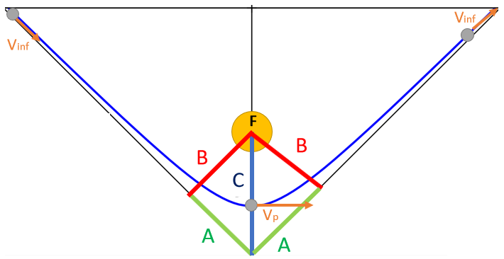
As with the elliptical orbit one has the periastre (perigee in the Earth system and perihelion in the solar system) is the point of orbit closest to the dominant body. The data couple at this point is the radius at the periastre rp and the velocity at the perastre vp
The hyperbole being open, there is no apoastre. On the other hand, in a case like an asteroid approaching the Earth it is necessary to calculate the risk of collision (including the periastre radius) before arriving at the periastre (and thus a collision). We therefore use the data between the so-called infinity system because are calculated for distances far removed from the dominant body. we define the velocity to infinity Vinf the velocity that the dominated body possesses by entering into the system of the dominat body. The second is the gap B between the asymptote and the focus. The asymptote is the axis that the object follows before entering the system and before being disturbed by the dominant body. The B gap is therefore the minimum distance between the dominant and dominated bodies if the dominant body had no gravitational influence.

Calculation
radius-velocity relationship
On a hyperbolic trajectory the velocity-raduis relationship still exists but is modified.

mu: standard gravitational parameter
r: radius
a: semi-major axis
Couple of data at the perastre
We can go from data to the perastre to geometric data we start by reversing the relationship radius-velocity to know a and then we deduce eccentricity e.

mu: standard gravitational paramete
vp: periastre velocity
rp: periastre radius

rp: periastre radius
a: semi-major axis
We can also calculate the geometrical data from the periastre data by calculating a semi-major axis and then using the radius-velocity relationship applied to the periastre.

a : semi-major axis
e : eccentricity

mu: standard gravitational parameterr
rp: periastrea radius:
a: semi-major axis
Data couple to infinity
We have a couple of data called “infinity” Vinf and B with parameters observable at the time of entry into the system. We can even anticipate much more, for example, by knowing the orbital parameters of an asteroid around the sun, we can know the parameters passing near the Earth decades in advance. we can calculate the semi-major axis directly with infinite velocity and then deduce the eccentricity with geometric relationships.

mu: standard gravitational parameter: Vinf: velocity at infinity

B: gap
:a semi-major axis
It is also possible to use direct relationships to calculate data at infinity with geometric parameters.

mu: gravitational parameter standard
a : semi-major axis

a: semi-major axis
e: eccentricity
direct perastre-infinite calculation
Thanks to more complex relationships, we can calculate the data at the periaastre directly with those to infinity, so we can judge the dangerousness of an asteroid, because if the radius to the periastra is less than the radius of the planet, there is impact and the energy of this impact depends on the velocity at the periastre.

mu: standard gravitational paramete
Vinf: velocity at infinity
B: gap

mu: standard gravitational parameterr
rp: periastre radius
vinf: velocity at infinity
We can also do the reverse calculation in order to know the conditions of exit system from the velocity given to an interplanetary probe from a parking orbit

vp: periastre velocity
mu: standard gravitational parameter
rp: periastre radius

mu: standardvinf gravitational parameter
Vinf: velocity at infinity:
rp: periastre radius
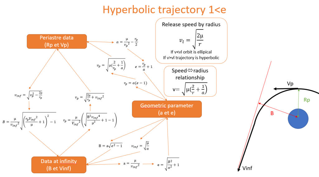
below is a summary of the formulas for past from one data couple to another.

In order to make everything is more concrete calculations and better understand their uses, here is a digital application